Parafermion Pictures

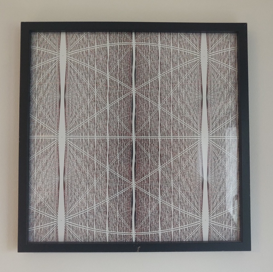
Parafermions are particles exhibiting parastatistics, thought to exist as excitations of exotic two dimensional materials and theorised to have useful applications in quantum information processing. Unlike Majorana fermions, systems of parafermions can potentially be used to realise fault tolerant quantum computation. In addition to this they can lead to some interesting pictures like the one above which is a framed print of one such picture. In this post I will go through the steps involved in creating such pictures along with the code to generate them. These came out of out of work which explored the properties of the energy spectra of parafermion chains [1].
We start with a model of particles occupying sites , each of which is labeled . The energy of the system only depends on the number and type of the particles and not the sites they occupy. This means that instead of looking at all possible ways of labeling all the sites, we can instead consider levels containing many configurations, all of which have the same energy. For example with two labels and four positions , there are five possible energy levels where the numbers of particles of each type are .
For general and , the number of energy levels is equal to the number of compositions of into parts. In the literature [2], this is denoted and are called extended binomial coefficients. They satisfy the recurrence relation
with and . A good way to think about these quantities and the recurrence relation is to picture the as denoting the number of ways of distributing items among boxes. If we imagine hovering over each box in turn and deciding whether or not to place an item in that box we can consider the possibilities which are:
We decide to place the item in the box, this results in items
remaining and still boxes to distribute among which gives the term
We decide not to place the item in the box, this means we still have items but now
only boxes to distribute them among which gives the term
With these recurrence relations it's possible to easily calculate the number of distinct energy levels for large systems. With memoization this can be made even more efficient. The following is simple Julialang function to calculate the number of levels for a given and
const cache = Dict{Tuple{Int, Int}, Int}()

function C_s(L, N)
    if haskey(cache, (L, N))
        return cache[(L, N)]
    elseif L == 1
        cache[(L, N)] = N
        return N
    elseif N == 1 || L == 0
        cache[(L, N)] = 1
        return 1
    else
        return C_s(L-1, N) + C_s(L, N-1)
    end
end
Using this function we evaluate the number of levels for a few different values of and to get:
| N | L=5 | L=10 | L=20 | L=30 |
|---|---|---|---|---|
| 2 | 6 | 11 | 21 | 31 |
| 3 | 21 | 66 | 231 | 496 |
| 4 | 56 | 286 | 1771 | 5456 |
| 5 | 126 | 1001 | 10626 | 46376 |
| 8 | 792 | 19448 | 888030 | 10295472 |
Which shows how quickly these numbers grow, particularly with large values. If we index each level with a integer in the range , then the same recurrence relation can be used to find the numbers of particles of each type for each index. We simple iterate through each of the positions and if the index is less than the first term, we place a particle at that position and continue with one less particle to be placed, if it is greater we move to the next position and subtract the first term from the index. The following function implements this.
function get_level(idx, L, N)
    @assert idx > 0 && idx <= C_s(L, N) "Index out of range"
    level = zeros(Int, N)
    pos = 1
    while pos < length(level) + 1 && L > 0 && idx > 0
        if idx <= C_s(L-1, N)
            level[pos] += 1
            L -= 1
        else
            pos += 1
            idx -= C_s(L-1, N)
            N -= 1
        end
    end
    level
end

# create generator from this function
get_levels(L, N) = (get_level(i, L, N) for i = 1:C_s(L, N))
For and we get the following levels
| idx | level |
|---|---|
| 1 | 4 0 0 |
| 2 | 3 1 0 |
| 3 | 3 0 1 |
| 4 | 2 2 0 |
| 5 | 2 1 1 |
| 6 | 2 0 2 |
| 7 | 1 3 0 |
| 8 | 1 2 1 |
| 9 | 1 1 2 |
| 10 | 1 0 3 |
| 11 | 0 4 0 |
| 12 | 0 3 1 |
| 13 | 0 2 2 |
| 14 | 0 1 3 |
| 15 | 0 0 4 |
Note that when retrieving all levels there are much more efficient approaches than the one above which make use of the fact that levels with consecutive indices are related.
Each particle type costs a different amount of energy which is a function of a parameter . A particle of type costs energy
This means that for some values of multiple particle types cost the same amount of energy and the orderings of energies get exchanged with changing theta. Given the particle composition of a level we can write a function to calculate the energy as
function energy(p, θ)
    N = length(p)
    -sum(p .* cos.(θ .+ 2π .* (1:N) ./ N))
end
We can use this function to plot the energies of the levels with changing . For each , the pattern will repeat every so to see the full pattern it is sufficient to look only in the interval . Below we show plots in this range for for small values of .
using Plots

function plot_energies(L, N)
    pl = plot()
    for p in get_levels(L, N)
        θs = range(0, stop=2π/N, length=50)
        pl = plot!(θs,
                   energy.([p], θs),
                   legend=false,
                   xlabel="θ",
                   ylabel="E",
                   title="N=$N")
    end
    pl
end

plot_N2 = plot_energies(5, 2)
plot_N3 = plot_energies(5, 3)
plot_N4 = plot_energies(5, 4)
From these and the numbers in the tables above we see that the plots get very busy for even modest and . The points where the bands cross have a special meaning for the physics of these systems so we now focus on finding these points from the level descriptions. For each pair of levels we find that they cross exactly twice in the interval . From the expression for the energy and a little algebra we can find the exact where two levels and cross is given by
where . Using this we can write a function to find the angle at which two levels cross as
function get_crossing(a, b)
    c = a - b
    N = length(a)
    θ = atan(sum(c .* cos.(2π / N .* (1:N))) /
             sum(c .* sin.(2π / N .* (1:N))))
    if θ < 0
        return θ + π
    else
        return θ
    end
end
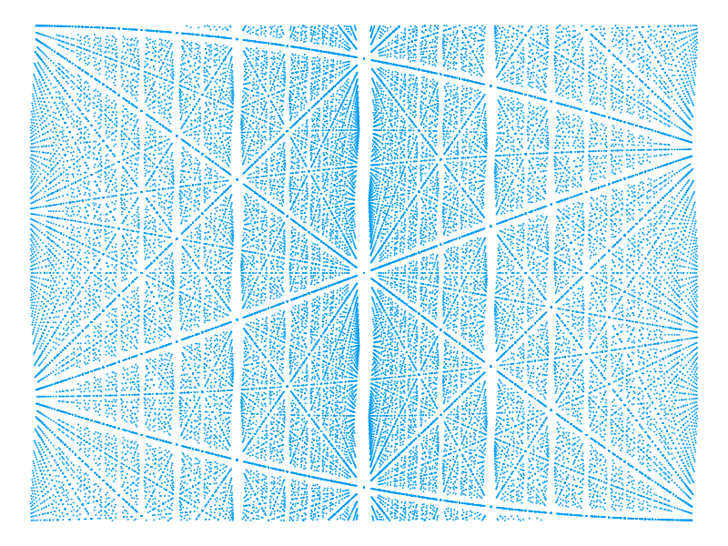
The Julialang atan function returns an angle in the range . We know that each pair of levels twice at angles radians apart so we adopt the convention that our get_crossing function will return the angle in the interval . The other crossing point can easily by found by subtracting from this. Using this function it's possible to pick out the crossings and plot these alone, making it possible to create plots for larger systems showing interesting patterns. The next example shows this being used for a relatively large system with and zooming in on a window of and values to show more detail. These windows values were selected because of the symmetry and density of crossings at this points.
function find_crossings(L, N, θ_window=nothing, E_window=nothing)
    levels = collect(get_levels(L, N));

    θs = Vector{Float64}()
    Es = Vector{Float64}()
    for (pos, a) in enumerate(levels)
        for b in levels[pos+1:end]
            θ = get_crossing(a, b)
            E = energy(a, θ)
            for θ′ in [θ-π, θ]
                if θ_window === nothing || (θ_window[1] <= θ′ <= θ_window[2])
                    if E_window === nothing || (E_window[1] <= E <= E_window[2])
                        push!(θs, θ′)
                        push!(Es, E)
                    end
                end
            end
        end
    end
    θs, Es
end

θs, Es = find_crossings(80, 3, [π/6 - 0.5, π/6 + 0.5], [-1, 1])

p = scatter(θs,
            Es,
            markershape=:circle,
            markersize=1.5,
            legend=nothing,
            markerstrokecolor=:auto,
            axis=nothing,
            xaxis=false,
            yaxis=false,
            size=(800, 600))
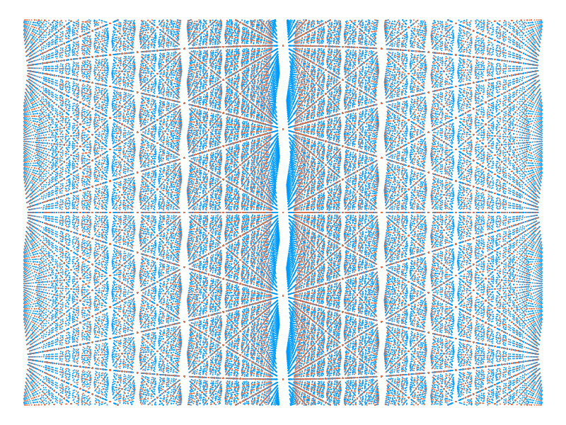
Another interesting direction to take is to use colour to distinguish the different types of crossing points. For example we can use the domain wall angle of the levels at each crossing to distinguish different crossings. This is a physical observable, defined in [1] which has important implications for the physics happening at each crossing. In the following we use different colours to distinguish crossings where the domain wall angles match and those where they differ.
function dw_angle(p)
    N = length(p)
    sum(p .* (1:N)) % N
end

function find_crossings(L, N, θ_window=nothing, E_window=nothing)
    levels = collect(get_levels(L, N));

    θs = Dict{Bool, Vector{Float64}}()
    Es = Dict{Bool, Vector{Float64}}()
    for (pos, a) in enumerate(levels)
        dwa_a = dw_angle(a)
        for b in levels[pos+1:end]
            key = dwa_a == dw_angle(b)
            θ = get_crossing(a, b)
            E = energy(a, θ)
            for θ′ in [θ-π, θ]
                if θ_window === nothing || (θ_window[1] <= θ′ <= θ_window[2])
                    if E_window === nothing || (E_window[1] <= E <= E_window[2])
                        if !haskey(θs, key)
                            θs[key] = Vector{Float64}()
                            Es[key] = Vector{Float64}()
                        end
                        push!(θs[key], θ′)
                        push!(Es[key], E)
                    end
                end
            end
        end
    end
    θs, Es
end

θs, Es = find_crossings(81, 3, [π/6 - 0.5, π/6 + 0.5], [-2, 2])

p = plot()
for key in keys(θs)
    global p = scatter!(θs[key],
                Es[key],
                markershape=:circle,
                markersize=1.5,
                legend=nothing,
                markerstrokecolor=:auto,
                axis=nothing,
                xaxis=false,
                yaxis=false,
                size=(800, 600))
end
The plots produced in this manner are rich in symmetries and other interesting features. By changing the system size and playing around with the parameter windows used, the aspect ratio, the thickness and type of symbols used, it's possible to create many interesting picture. A github gist with the full source code which provides a good starting point is available here. It's best to run this script with a recent version of Julialang (recommended 1.5.x or greater) with the Plots.jl package installed. Further details and background on the physics of these systems can by found in the papers [1], [3] and the references therein.
| [1] | Phys. Rev. B 95 235127 (2017) |
| [2] | http://citeseerx.ist.psu.edu/viewdoc/summary?doi=10.1.1.397.3745 |
| [3] | https://arxiv.org/abs/1908.03459 |